

Before we test any strategy, we need a foundation: a consistent way to load data, compute returns, and run backtests that we can reuse across every post in this series.
This post is intentionally technical. It’s the plumbing. But if you build it properly now, every post that follows becomes dramatically simpler, you’ll be writing strategy logic, not boilerplate.
By the end of this post you’ll have a Strategy base class that handles data loading, return computation, position management, and performance reporting. We’ll use it for every single backtest from post 1.1 onwards.
The data structure: OHLCV
Your data almost certainly comes in OHLCV format:
We'll almost always use the Close price for signal construction. A note on why: using High or Low to construct signals and then assuming you traded at Close introduces look-ahead bias — you're using information from within the candle that wasn't available at the open. For simplicity and cleanliness, Close-to-Close is the standard.
Simple returns vs log returns
This distinction matters and it's worth understanding properly.
Simple return:
Log return:
Why do we prefer log returns for backtesting?
Three reasons:
Time additivity. Log returns add across time. If BTC returned 5% on Monday and 3% on Tuesday, your log return over the two days is 5% + 3% = 8% (approximately). Simple returns don’t add — they compound. This makes multi-period calculations much cleaner.
Statistical properties. Log returns are closer to normally distributed than simple returns. This matters when you apply statistical tests — many assume normality, and while crypto returns are still fat-tailed, log returns are better-behaved.
Symmetry. A −50% simple return requires a +100% return to recover. A −50% log return requires a +50% log return. Symmetry makes mathematical analysis cleaner.
One important note: when reporting results to humans, convert back to simple returns. Log returns of 15% don’t mean 15% profit — they mean e^0.15 − 1 = 16.2% profit. For communication, use simple. For computation, use log.
The base class
Here's the foundation we'll build on. Every strategy in this series will inherit from this:
import numpy as np
import pandas as pd
from dataclasses import dataclass, field
from typing import Optional

@dataclass
class BacktestResult:
    equity:       pd.Series
    returns:      pd.Series
    positions:    pd.Series
    sharpe:       float
    sortino:      float
    max_dd:       float
    ann_return:   float
    ann_vol:      float
    win_rate:     float
    n_trades:     int

class Strategy:
    """
    Base class for all strategies in this series.
    Inherit from this and implement `generate_signal()`.
    """

    def __init__(
        self,
        prices:    pd.DataFrame,      # OHLCV DataFrame, index = DatetimeIndex
        costs:     float = 0.001,     # 10bps per trade (one-way)
        freq:      int   = 252,       # trading days per year
    ):
        self.prices  = prices
        self.close   = prices['close'] if 'close' in prices.columns else prices['Close']
        self.costs   = costs
        self.freq    = freq
        self.returns = np.log(self.close).diff().dropna()   # log returns

    def generate_signal(self) -> pd.Series:
        """
        Override in subclass.
        Returns a Series of {-1, 0, 1} aligned to self.returns.index.
        -1 = short, 0 = flat, 1 = long.
        """
        raise NotImplementedError

    def run(self) -> BacktestResult:
        signal   = self.generate_signal()
        position = signal.shift(1).reindex(self.returns.index).fillna(0)
        turnover = position.diff().abs().fillna(0)

        strat_ret = position * self.returns - turnover * self.costs
        equity    = (1 + strat_ret.apply(lambda x: np.exp(x) - 1)).cumprod()

        return self._compute_stats(strat_ret, equity, position)

    def _compute_stats(self, ret, equity, position) -> BacktestResult:
        ann_ret  = ret.mean() * self.freq
        ann_vol  = ret.std()  * np.sqrt(self.freq)
        sharpe   = ann_ret / ann_vol if ann_vol > 0 else 0

        neg_ret  = ret[ret < 0]
        sortino  = ann_ret / (neg_ret.std() * np.sqrt(self.freq)) if len(neg_ret) > 0 else 0

        rolling_max = equity.cummax()
        max_dd      = ((equity - rolling_max) / rolling_max).min()

        trades    = position.diff().abs()
        n_trades  = int((trades > 0).sum())
        win_rate  = (ret[position.shift(1) != 0] > 0).mean()

        return BacktestResult(
            equity     = equity,
            returns    = ret,
            positions  = position,
            sharpe     = round(sharpe, 3),
            sortino    = round(sortino, 3),
            max_dd     = round(max_dd, 4),
            ann_return = round(ann_ret, 4),
            ann_vol    = round(ann_vol, 4),
            win_rate   = round(win_rate, 3),
            n_trades   = n_trades,
        )

    def plot(self, result: BacktestResult, title: str = 'Strategy'):
        import matplotlib.pyplot as plt
        import matplotlib.gridspec as gridspec

        fig = plt.figure(figsize=(12, 7))
        gs  = gridspec.GridSpec(3, 1, height_ratios=[0.15, 0.55, 0.30], hspace=0.08)

        # -- metrics header
        ax0 = fig.add_subplot(gs[0])
        ax0.axis('off')
        metrics = (
            f"Sharpe: {result.sharpe:.2f}  |  "
            f"Sortino: {result.sortino:.2f}  |  "
            f"Ann. Return: {result.ann_return*100:.1f}%  |  "
            f"Ann. Vol: {result.ann_vol*100:.1f}%  |  "
            f"Max DD: {result.max_dd*100:.1f}%  |  "
            f"Win Rate: {result.win_rate*100:.0f}%  |  "
            f"Trades: {result.n_trades}"
        )
        ax0.text(0, 0.5, title, fontsize=14, va='center', fontweight='normal')
        ax0.text(0, 0.0, metrics, fontsize=9, va='center', color='#888')

        # -- equity curve
        ax1 = fig.add_subplot(gs[1])
        result.equity.plot(ax=ax1, color='#7ec8a4', linewidth=1.4)
        ax1.axhline(1, color='#333', linewidth=0.5, linestyle='--')
        ax1.set_ylabel('Portfolio value', fontsize=9)
        ax1.tick_params(labelbottom=False)

        # -- drawdown
        dd = (result.equity / result.equity.cummax() - 1) * 100
        ax2 = fig.add_subplot(gs[2], sharex=ax1)
        ax2.fill_between(dd.index, 0, dd.values, color='#d4756b', alpha=0.6)
        ax2.set_ylabel('Drawdown %', fontsize=9)

        plt.tight_layout()
        return fig
Loading your data
If your data is in CSV format, one file per coin:
import os

def load_universe(data_dir: str, coins: list) -> dict:
    """
    Load OHLCV data for multiple coins.
    Returns dict: {'BTC': DataFrame, 'ETH': DataFrame, ...}
    """
    universe = {}
    for coin in coins:
        path = os.path.join(data_dir, f'{coin}.csv')
        df   = pd.read_csv(path, index_col=0, parse_dates=True)
        df.columns = df.columns.str.lower()
        df   = df[['open','high','low','close','volume']].dropna()
        universe[coin] = df
    return universe

# Usage
coins    = ['BTC', 'ETH', 'BNB', 'SOL', 'ADA',
            'XRP', 'DOT', 'AVAX', 'LINK', 'MATIC']
universe = load_universe('./data', coins)
A quick sanity check
Before you run any backtest, always do these three checks:
def sanity_check(universe: dict):
    for coin, df in universe.items():
        print(f"\n{coin}")
        print(f"  Period : {df.index[0].date()} → {df.index[-1].date()}")
        print(f"  Rows   : {len(df)}")
        print(f"  NaNs   : {df.isnull().sum().sum()}")
        print(f"  Gaps   : {(df.index.to_series().diff().dt.days > 1).sum()} missing days")

        # check for zero or negative prices (data error)
        if (df['close'] <= 0).any():
            print(f"  ⚠️  WARNING: zero or negative close prices detected")

sanity_check(universe)
Data problems that will silently ruin a backtest: duplicate timestamps, missing days without NaN (filled with previous close), split-adjusted prices mixing with unadjusted, and timezone mismatches. Check before you assume.
Using the base class
Here's how every future strategy will look. Post 1.2, for example:
class SMA_Crossover(Strategy):

    def __init__(self, prices, fast=10, slow=30, **kwargs):
        super().__init__(prices, **kwargs)
        self.fast = fast
        self.slow = slow

    def generate_signal(self) -> pd.Series:
        fast_ma = self.close.rolling(self.fast).mean()
        slow_ma = self.close.rolling(self.slow).mean()
        signal  = pd.Series(0, index=self.close.index)
        signal[fast_ma > slow_ma] =  1
        signal[fast_ma < slow_ma] = -1
        return signal.reindex(self.returns.index)

# Run it
btc     = universe['BTC']
strat   = SMA_Crossover(btc, fast=10, slow=30, costs=0.001)
result  = strat.run()
fig     = strat.plot(result, title='BTC — SMA(10,30) Crossover')

print(f"Sharpe: {result.sharpe}")
print(f"Max DD: {result.max_dd:.1%}")
Clean, reusable, consistent across every strategy we test.
I run a simple example on the daily data of SOL/USDT using the above Sma_Crossover class using 1 Day and 1 week for respectively the fast and slow moving average.
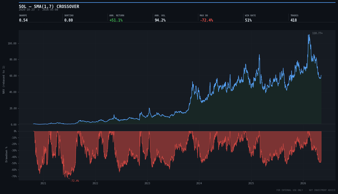
To illustrate how the class works, I ran a simple example on daily Solana/Tether data using the Sma_Crossover class, with a 1-day fast moving average and a 1-week slow moving average. For now, don’t focus on the strategy results, the goal here is simply to show how the implementation works in practice.
What’s next
Post 0.3 is the most important post in this series before we test anything real. We’re going to generate completely random trading signals and run them through this exact base class. The result is a distribution of Sharpe ratios under the null hypothesis, pure noise.
Every strategy from post 1.1 onwards has to beat that distribution to be considered real. If it doesn’t, we discard it regardless of how good the in-sample backtest looks.
That’s the scientific standard we’re setting. See you there.